Editing Log Data
This tutorial will cover feature of LogView++ to deal with las file, including import, export, doing calculation of log data, making partial log, and combining log data.. This is the basic operation that everybody need to understand before dealing with complicated graphical plotting and cross-sectioning.
Format File
Supported format file in LogView++ version 2012.2 is still LAS 2.0. Other LAS version might resulting unexpected result. LAS 2.0 must have at least the following keywords in the header file:
~Version Information
VERS. 2.0:
WRAP. NO:
~Well Information
~Curve Information
DEPT. :
~Other information
~A
Remarks:
~Version Information, gives the version of the LAS format and wrapping mode. Make sure the format is 2.0. Wrapping true means that the data (in the ~A section) in the log is formatted in multi-line rather than single line.
~Well Information, usually includes the well identification like well name, start depth of log and etc.
~Curve Information, should includes all column data name exists in the file. At least, it should contain DEPT.
~A or ~Asci Data Section, is the final section that filled up with all numerical values of the log data. Number of column must be equal to the number of column defined in the ~Curve Information.
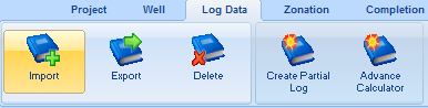
Basic Operation of LAS File
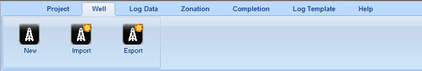
Importing LAS File
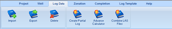
This is simple. But, be AWARE, some people made a mistake by choosing wrong menu. Please choose menu “Log Data” and “Import”. DO NOT USE MENU FROM “Project” or “Well” !!!!!!
After clicking that menu, browse a valid LAS file, and open. You will be prompted with this dialog..
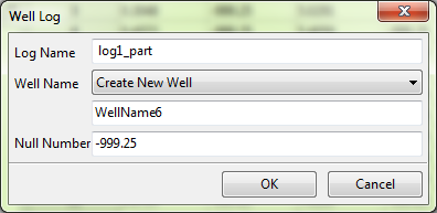
Give a name, and decide whether this imported log would be a part of specific well or just create new well for it. This null number is actually magic number that is defined to accommodate the NULL number in log file. Default value is -999.25 (I don’t know why somebody choose that strange number.. 🙂 )
Just click OK and done!!.
Exporting LAS File
It can be done simply by going to menu “Log Data” and select “Export”. You must be prompted by a dialog. Select the proper well and the log, and export. Done.. Nothing complicated.
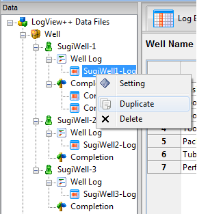
Renaming, Duplicating, and Deleting the Log
Right click in the main data tree as shown below, select Setting for renaming, Duplicate for duplicating, and surely Delete for deleting.
You must noted that deleting a log data or anything would be allowed in case of the data is not being used by any of window or editor.
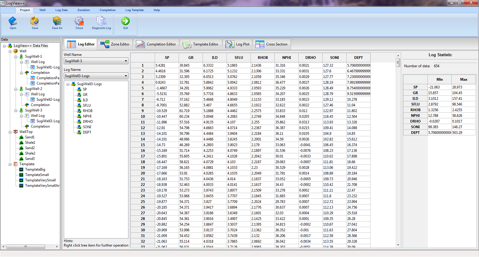
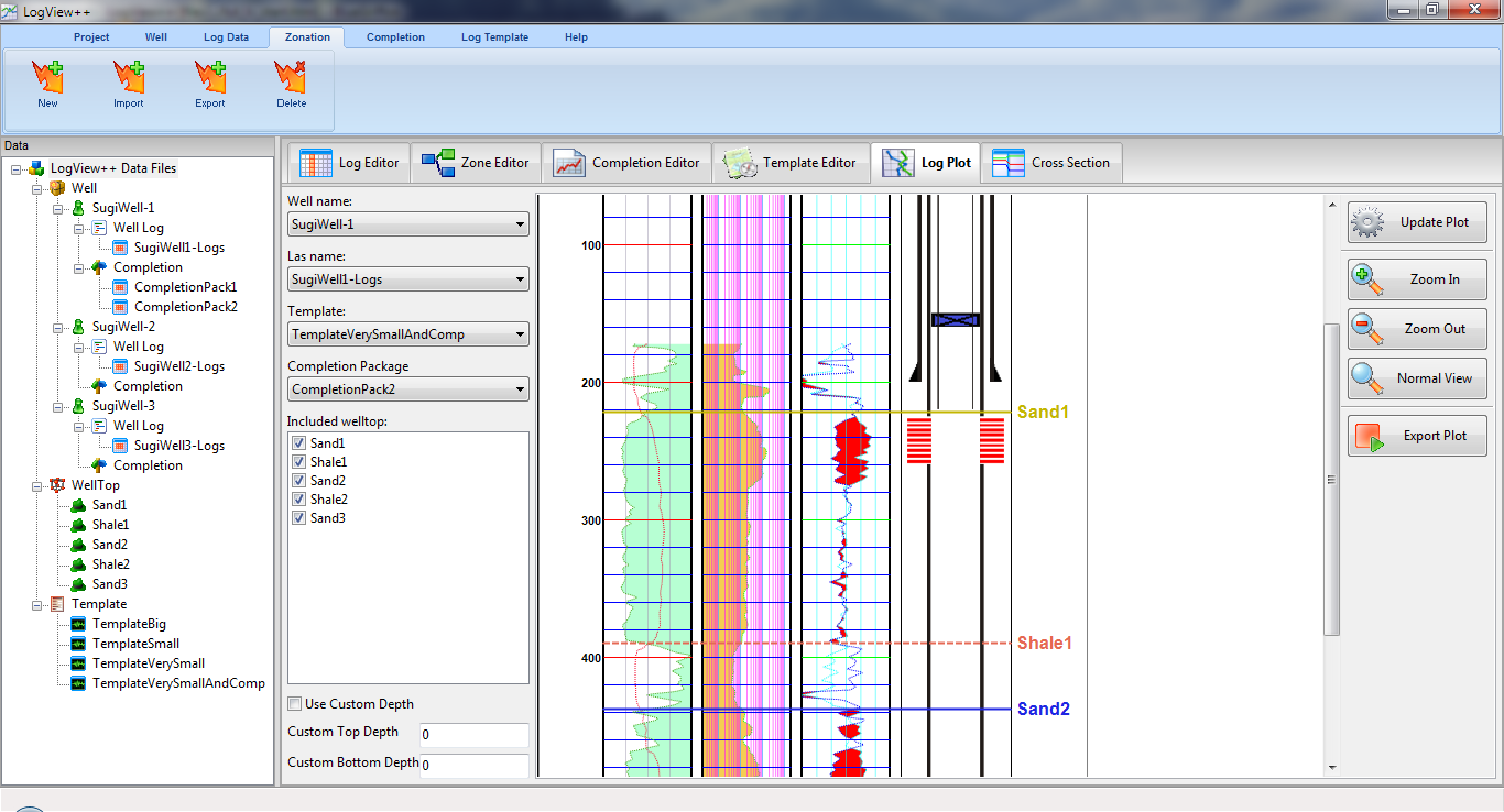
Showing Imported Las File
To show the imported LAS File, simply go to tab Log Editor, then select well name and las name to be shown. Correct operation should give this kind of screenshot.

This log editor shows the tree of data available in the log, table of all data, and also statistic data of each column that should be useful for determining the limit of value in the next plotting procedure.
Editing Imported Las File
Rename & Delete Column
It can be simply done by right click the tree of log data and select menu rename or delete…
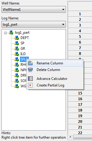
Create Partial Log
Creating a part of log sometimes is very important especially if we want to calculate a certain interval that have a very different property compared to whole log interval. To do that, right click tree data, and select “Create Partial Log”. You will get to this kind of dialog. 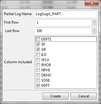
Those dialog is example if we want to make a partial log of the existing log data, only for the first 100 rows, and only for column SP, GR, and DEPT. By clicking “Create”, you will have new partial log data in the same well as the original log from. To show the partial log, just do select the new well log in the log editor window.
Advance Calculator
I call it advance because of this is probably the most difficult operation and the most useful feature in this editing the Las file chapter. Right click on tree, and select menu “Advance Calculator”. And you will see this kind of dialog.
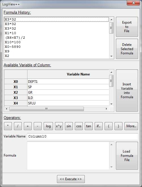
This dialog contain 3 parts which are formula history, variables, and formula to be calculated. The formula history shows any formula that you ever calculate previously. To re-calculate again the previous calculation, just double click the history and you will get your formula in the form.
Variables shows all data column available in the selected las file and its aliases. For example, in above picture, rows no-1 shows X0 and DEPT1. That means the column name is DEPT1 and the alias is X0. !!!PLEASE BE CAREFUL!!!. You are only allowed to use the alias in the formula, not the real name.
In the formula section, it has operator, variable name, and formula itself. Operator is operator.. 🙂 like +, – , log, and etc. Variable name is the expected result column name. and the formula is of course the equation to be calculated. We can write formula single line or multi-line format. And it could be a very complicated formula if you wish. Please take a look at this example formula.
single line formula:
if(X0>1000 & X1!=-999.25, X1/100, -999.25)
——————————————
it should clearly explained.. 🙂
multi-line formula:
A:=X0;
B:=X1;
C:=A+B;
C
——————————————
first and second line, we make new sub variable called A & B.
third line, C is derived from A & B
last line, C is return as final result.
We can also write as follows…
——————————————
A:=X0;
B:=X1;
A+B
——————————————
those 2 example will give same result & same meaning actually.. 🙂 If you you want to know more about the supported operator, please click “More” for further documentation. After formula is ready, click “Execute”, and you will have new column data in the table. Enjoy it..
Combining Two Log Data
Combining two log data is also one of the difficult task to do since sometime a little bit confusing. More over, I have no enough time to test this feature. So, probably you will encounter an unexpected bug while doing this.
For example, we have 2 partial data like this:
Las File – 1:
Las File – 2:
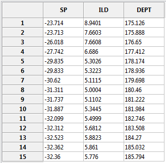
We want to combined those two files to become one file for simplicity.
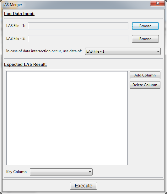
To do that, go to menu bar “Log Data” and select “Combine LAS Files”. By doing that, you will be prompted by this kind of dialog. Browse LAS File – 1 and 2 from the dialog. By default, in case of data intersection occur, it will used data from LAS File-1. But actually you can change it to LAS File – 2 as well.
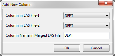
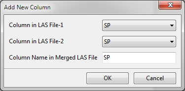
Once two LAS Files ready, click “Add Column” and select the appropriate column pairs for those two LAS Files. Figure below shows how to add 4 column in the targeted merged file. In the first 2 pictures, it shows pairs that both Las File – 1 and 2 are having the column. In the second row, the GR column is not available in the Las File-2. So we can choose NULL for that. The ILD is also not available in the Las File – 1. So we can also choose the NULL for that.
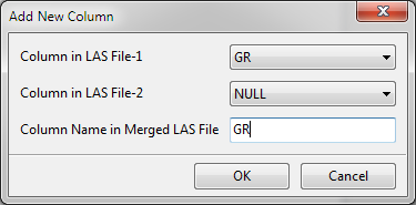
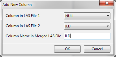
After all columns are ready, last but the most important thing is that we must specify the Key Column. This is the column that both Las File-1 and 2 have it and will be used for reference of merging. Ideally, this Key Column should be the DEPT since we want to merge mainly for the depth.
After we finish the merging setup. Click execute and you will prompted to save the resulted file. And you can imported to the LogView++ to compare the result with the data source. Doing the correct procedure should give this kind of result.
 This is the end of this tutorial. Should anybody have question, please don’t hesitate to contact my email.
——————————————————————–
Written by Sugiyanto Suwono
Bekasi, March 12, 2013

 and you will be prompted with this kind of dialog. Fill the name of the data, let say “Data1_Training” and click OK.