The final step of AgielNN is forecasting. This should be the easiest process in AgielNN. After finished douing some training and checking; and going with best match to actual data; forecasting can be made using the model by taking a step to “Forecasting” tab in AgielNN.Before that, make sure you are not bypassing the data preparation for forecasting as explained in the first tutorial of data preparation.

There are 2 choices we have to do the process.

Case 1: Use the matched model.

1. In this case, you can simple select the “Use latest trained ANN” (selected by default).
2. Select the data to be used in the combo box of “Data used”
3. Select a number of column as input. Be sure that the number of column must be equal to the number of column used during training and checking.
4. Click “Do Forecast”

Case 2: Use saved AgielNN model.

1. In this case, select the “Use other ANN file”.
2. Browse the ANN model saved from previous training and checking.  The ANN file model must be a model exported from AgielNN and should have *.ann extension. It is not compatible with another ANN file generated by another neural network software. The file can be exported thru menu File — Export — Artificial Neural Network — ANN Trained Model.
3. Select the data to be used in the combo box of “Data used”
4. Select a number of column as input. Be sure that the number of column must be equal to the number of column used during training and checking.
5. Click “Do Forecast”

The screenshot of the software should be like this.

—————————————————————-

This is the end of tutorial. Should anybody have question, please mail me. Thanks.
Written by: Sugiyanto
28 June 2013.

Continuing the previous tutorial about neural network setup, now we have ready neural network model. To do a training and checking, please go to tab “Training Run”. There is nothing complicated here. All default parameters are already set. If you don’t have any idea about parameters; as i am he he…; just click “Do Train” and hopefully all of the problem solved..

However, in some cases, this simple training process is not that easy as it is looked. So, somehow, you might need to modify the value of those parameters to get the best solution.

Since I don’t have any clue at all about the parameters, here i would directly refers to FANN documentation as follows. Somebody with good mathematical background should understand better on this 🙂

Source: “fann_data.h”

—————————————–

The Training algorithms used when training. The incremental training looks alters the weights after each time it is presented an input pattern, while batch only alters the weights once after it has been presented to all the patterns.

## FANN_TRAIN_INCREMENTAL

Standard back-propagation algorithm, where the weights are updated after each training pattern. This means that the weights are updated many times during a single epoch. For this reason some problems, will train very fast with this algorithm, while other more advanced problems will not train very well.

## FANN_TRAIN_BATCH

Standard back-propagation algorithm, where the weights are updated after calculating the mean square error for the whole training set. This means that the weights are only updated once during a epoch. For this reason some problems, will train slower with this algorithm. But since the mean square error is calculated more correctly than in incremental training, some problems will reach a better solutions with this algorithm.

## FANN_TRAIN_RPROP

A more advanced batch training algorithm which achieves good results for many problems. The RPROP training algorithm is adaptive, and does therefore not use the learning_rate. Some other parameters can however be set to change the way the RPROP algorithm works, but it is only recommended for users with insight in how the RPROP training algorithm works. The RPROP training algorithm is described by [Riedmiller and Braun, 1993], but the actual learning algorithm used here is the iRPROP- training algorithm which is described by [Igel and Husken, 2000] which is an variety of the standard RPROP training algorithm.

## FANN_TRAIN_QUICKPROP

A more advanced batch training algorithm which achieves good results for many problems. The quickprop training algorithm uses the learning_rate parameter along with other more advanced parameters, but it is only recommended to change these advanced parameters, for users with insight in how the quickprop training algorithm works. The quickprop training algorithm is described by [Fahlman, 1988].”
——————————————
The activation functions used for the neurons during training. The activation functions can either be defined for a group of neurons by <fann_set_activation_function_hidden> and <fann_set_activation_function_output> or it can be defined for a single neuron by <fann_set_activation_function>. The steepness of an activation function is defined in the same way by <fann_set_activation_steepness_hidden>, <fann_set_activation_steepness_output> and fann_set_activation_steepness>.

The functions are described with functions where:
* x is the input to the activation function,
* y is the output,
* s is the steepness and
* d is the derivation.

FANN_LINEAR – Linear activation function.
* span: -inf < y < inf
* y = x*s, d = 1*s
* Can NOT be used in fixed point.

FANN_THRESHOLD – Threshold activation function.
* x < 0 -> y = 0, x >= 0 -> y = 1
* Can NOT be used during training.

FANN_THRESHOLD_SYMMETRIC – Threshold activation function.
* x < 0 -> y = 0, x >= 0 -> y = 1
* Can NOT be used during training.

FANN_SIGMOID – Sigmoid activation function.
* One of the most used activation functions.
* span: 0 < y < 1
* y = 1/(1 + exp(-2*s*x))
* d = 2*s*y*(1 – y)

FANN_SIGMOID_STEPWISE – Stepwise linear approximation to sigmoid.
* Faster than sigmoid but a bit less precise.

FANN_SIGMOID_SYMMETRIC – Symmetric sigmoid activation function, aka. tanh.
* One of the most used activation functions.
* span: -1 < y < 1
* y = tanh(s*x) = 2/(1 + exp(-2*s*x)) – 1
* d = s*(1-(y*y))

FANN_SIGMOID_SYMMETRIC – Stepwise linear approximation to symmetric sigmoid.
* Faster than symmetric sigmoid but a bit less precise.

FANN_GAUSSIAN – Gaussian activation function.
* 0 when x = -inf, 1 when x = 0 and 0 when x = inf
* span: 0 < y < 1
* y = exp(-x*s*x*s)
* d = -2*x*s*y*s

FANN_GAUSSIAN_SYMMETRIC – Symmetric gaussian activation function.
* -1 when x = -inf, 1 when x = 0 and 0 when x = inf
* span: -1 < y < 1
* y = exp(-x*s*x*s)*2-1
* d = -2*x*s*(y+1)*s

FANN_ELLIOT – Fast (sigmoid like) activation function defined by David Elliott
* span: 0 < y < 1
* y = ((x*s) / 2) / (1 + |x*s|) + 0.5
* d = s*1/(2*(1+|x*s|)*(1+|x*s|))

FANN_ELLIOT_SYMMETRIC – Fast (symmetric sigmoid like) activation function defined by David Elliott
* span: -1 < y < 1
* y = (x*s) / (1 + |x*s|)
* d = s*1/((1+|x*s|)*(1+|x*s|))

FANN_LINEAR_PIECE – Bounded linear activation function.
* span: 0 <= y <= 1
* y = x*s, d = 1*s

FANN_LINEAR_PIECE_SYMMETRIC – Bounded linear activation function.
* span: -1 <= y <= 1
* y = x*s, d = 1*s

FANN_SIN_SYMMETRIC – Periodical sinus activation function.
* span: -1 <= y <= 1
* y = sin(x*s)
* d = s*cos(x*s)

FANN_COS_SYMMETRIC – Periodical cosinus activation function.
* span: -1 <= y <= 1
* y = cos(x*s)
* d = s*-sin(x*s)

FANN_SIN – Periodical sinus activation function.
* span: 0 <= y <= 1
* y = sin(x*s)/2+0.5
* d = s*cos(x*s)/2

FANN_COS – Periodical cosinus activation function.
* span: 0 <= y <= 1
* y = cos(x*s)/2+0.5
* d = s*-sin(x*s)/2

Source: “fann_train.h”

———————————

The learning rate is used to determine how aggressive training should be for some of the training algorithms (FANN_TRAIN_INCREMENTAL, FANN_TRAIN_BATCH, FANN_TRAIN_QUICKPROP). Do however note that it is not used in FANN_TRAIN_RPROP. The default learning rate is 0.7

Maximum epoch basically maximum number of trials to be conducted. The bigger value of maximum epoch should give the longer running time. Expected error is the targeted error to be pursued. The smaller value of expected error should also give the longer running time. And in many cases, this expected error somehow will never be achieved. So, don’t worry if you have never achieve a good expected error.

Actually, there are many parameters of FANN that have not yet supported in this version of AgielNN. If you like to know more about that, I really recommend you to directly access the FANN documentation. However, i am still working with the next version of AgielNN, so hopefully most of parameters of FANN could be supported in the next AgielNN releases.

Anyway, after you finish “playing” with parameters, please click “Do Training”. And you should get the comparison of training data vs training result, checking data vs checking result, in form of table and chart as show in this example.

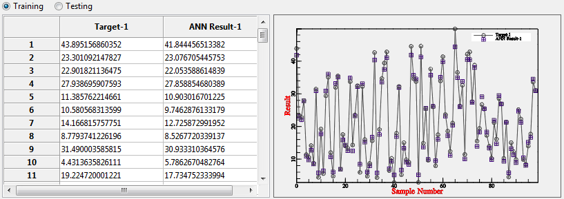
Using those kind of result comparison, it might be easier to decide whether the training is “enough” or still need more training process.

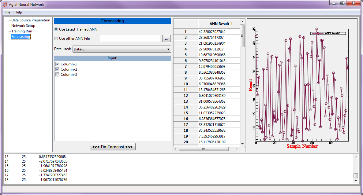
And also one of the important result from this training process is the Training logs that is printed in the bottom part of the software. This log basically tells everything about steps of training process, including the final result of weights and biases.

So, the training and checking is basically finished. But again, this procedure might need to be conducted back and forth with network setup to make sure of getting the best match to real data.

This is the end of this tutorial. Should anybody have question, please don’t hesitate to contact my email.
——————————————————————–
Written by Sugiyanto Suwono
Bekasi, April 30, 2013