Tutorial 1: Safira Digitizer

All Safira Digitizer task can simply be accessed by the toolbar as shown above.

  • Creating New Project
    Creating new project is one of the simplest task in Safira Digitizer. It will close the existing opened project and start with new blank project. To do that, simply click the toolbar “New Project” or menubar File-New Project.
  • Opening Existing Project
    This will open the saved Safira Digitizer project (*.sfd). Click toolbar “Open Project” or menubar File-Open Project” and browse to the saved file. To test whether Safira Digitizer correctly running or not, you can open sample projects exists in folder “samples”.
  • Saving Project
    Saving the project can be done by clicking toolbar “Save Project” or “Save Project As” or its menubar. You will be prompted to choose a new project filename.
  • Importing image
    Importing image in most cases is the first important step to start digitizing. Click toolbar “Import Image” and browse existing image to be digitized. The file format could be *.png, *.bmp, *.gif, or *.jpeg”. Once it is imported, the image will be plotted in the view panel.
  • Calibrating Image
    Calibrating image is a process to make Safira Digitizer understand the real coordinate of the image. Without calibration, Safira Digitizer will directly use the exact value from the screen coordinate. Therefore, the result might be away different from the real coordinate. This calibration can be done by clicking toolbar “New Calibration” and calibration dialog will be shown up. You must read carefully the notes in the bottom part of the dialog as follows:

    To calibrate the coordinate:
    1. Make sure the imported image is on correctly horizontal position.
    2. Select 2 points (X1,Y1) and (X2,Y2) that have different X values and Y values as like as above sample picture.

    Those notes should clearly explain how to do the next procedure.. Just click OK and select 2 coordinate for calibration. To ease the calibration, it is suggested to select 2 points that is located at the maximum value of X and Y, for example at (0,Ymax) and (Xmax, 0). Once the 2nd point is clicked, this following message box should be prompted.

    Click Ok and go to setting panel to change the real X and Y values of those 2 selected points.

  • Setting Up the View
    The following value in the setting panel can be adjusted to change the appearance of the viewer panel.

    1. Bitmap Angle
      Changing this value will rotate the bitmap as the value of angle. This is important in some condition where the image is not exactly positioned at horizontal position.
    2. Show Grid
      It is intended to change the grid plot in the viewer plot. It can be selected between “both”, “X-Axes”, “Y-Axes”, or “None”
    3. X-Axes Scale
      It is a choice of linear or logarithmic scale for X-axes.
    4. Y-Axes Scale
      It is a choice of linear or logarithmic scale for Y-axes.
    5. Decimal
      It is the precission value to be shown. The higher the value the more precise the number.
    6. Package Shown
      It is a choice whether to show only the selected package or to show all packages.
  • Creating Data Package
    Data package is a group / table that can contain many of points picked from the image. A project file can contain many data packages. To create a package, click toolbar “Add Package” and give a name of the package. It must be noted that you cannot pick any points from the point unless a package has been created.
  • Deleting Data Package
    Deleting package is certainly to remove a package from the project. It can be done by selecting the package and click toolbar “Delete Package”.
  • Picking Data
    After creating new package, you can start picking points in the viewer panel. To do that, first you have to click button “Pick Mode” and that click inside the viewer panel. A new point clicked will automatically generated inside the Data Package table.
  • Editing Data
    1. Insert New Points
      To insert new point between data in a package, first, you have to select a row in the data package table. The selected point will be highlighted in the viewer panel. Next step, click button “Pick Mode” and click new point to be inserted after the highlighted point.
    2. Deleting Points
      Similar to insertion, first you have to select rows to be deleted inside the data table, and then simply click Del in your keyboard.
  • Exporting Data
    Exporting data is one of the most important step in Safira Digitizer. It will export all packages and points inside the package as a text file. After that, it can be imported to other program i.e EXCEL for further usage / calculation. To do that, click toolbar “Export Data” and fill the new filename to dump the data. The exported file should be formated like this:

    Those exported data contains 2 packages (Curve-1 and Curve-2) and each package has its a bunch of real X and Y values.

 

Tutorial 1: IstiChartLib Basic

In this tutorial, I will show how simple is IstiChartLib for making simple plot.

Generally, the library consist of 6 Classes:

  1. istiChartAxis, for customizing axis
  2. istiChartLegend, for customizing the legend
  3. istiChartMarker, for customizing chart series marker
  4. istiChartPanel, panel for plotting the chart
  5. istiChartSeries, series of data to be plotted, and
  6. istiChartXY, the chart itself

For making simple chart, we dont have to deal with all of them. Simply use the istiChartPanel. Please see the following Test1 sample in IstiChartDemo code:


1   istiChartPanel *chart1 = new istiChartPanel(pnlCommonXY);
2   wxBoxSizer *box1 = new wxBoxSizer(wxHORIZONTAL);
3   box1->Add(chart1, 1, wxEXPAND);
4   pnlCommonXY->SetSizer(box1);

5   chart1->GetChart().SetTitle(“Common XY Chart Demo”);
6   for (int x = 0; x < 20; x++) {
7      istiChartSeries seri(“Chart-” + toString(x+1, -1));
8      VectorDouble VX, VY;
9      for (int i = 0; i <= 1000; i++) {
10         VX.push_back((double)i/10); //Data X
11         VY.push_back((x+1)*sin((double)i/10.0/(x+5)*PHI)); //Data Y
12     }
13     seri.SetData(VX, VY);
14     chart1->GetChart().AddSeries(seri);
15  }
16  chart1->GetChart().GetLegend()->SetMaximumColumn(2);
17  chart1->Update();


line 1-4:  It is making istiChartPanel as a child of pnlCommonXY. It is actualy as simple as wxPanel in general. Don’t be bothered with pnlCommonXY. It can be any wxPanel or even your main wxFrame.

Line 5:  Create the title of the chart

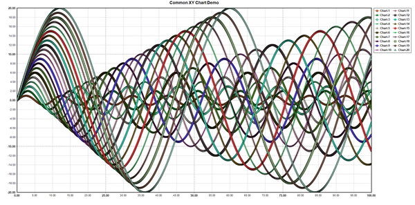
Line 6-15: It is used to make 20 chart series and adding the series to the chart. Each series has 1000 data of X and Y that is stored in VectorDouble VX and VY which is actually similar to vector<double> in std C++ library.

Line 16:  Make the legend to have 2 column

Line 17: Draw the chart.


If nothing wrongs occur, the result should be like this:

IstiChartLib


Written by: Sugiyanto Suwono

Januari 26, 2016

Tutorial 4: AgielNN Forecasting

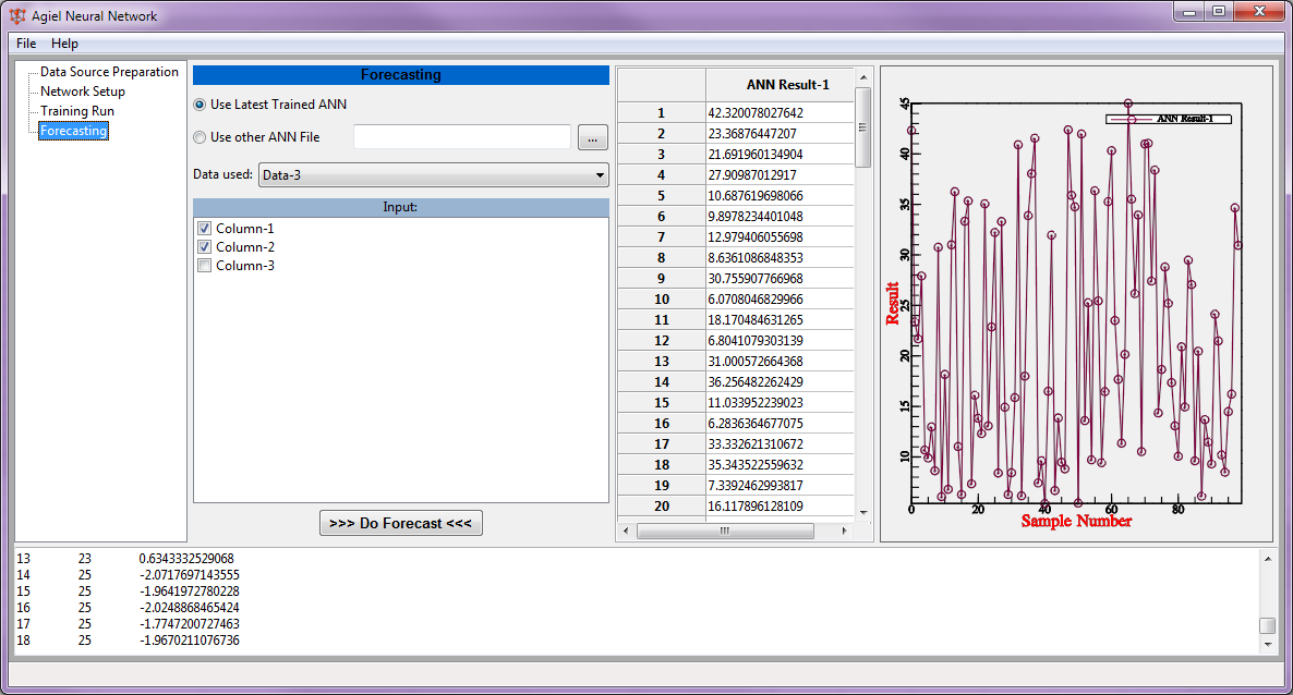
The final step of AgielNN is forecasting. This should be the easiest process in AgielNN. After finished douing some training and checking; and going with best match to actual data; forecasting can be made using the model by taking a step to “Forecasting” tab in AgielNN.Before that, make sure you are not bypassing the data preparation for forecasting as explained in the first tutorial of data preparation.

There are 2 choices we have to do the process.

Case 1: Use the matched model.

  1. In this case, you can simple select the “Use latest trained ANN” (selected by default).
  2. Select the data to be used in the combo box of “Data used”
  3. Select a number of column as input. Be sure that the number of column must be equal to the number of column used during training and checking.
  4. Click “Do Forecast”

Case 2: Use saved AgielNN model.

  1. In this case, select the “Use other ANN file”.
  2. Browse the ANN model saved from previous training and checking.  The ANN file model must be a model exported from AgielNN and should have *.ann extension. It is not compatible with another ANN file generated by another neural network software. The file can be exported thru menu File — Export — Artificial Neural Network — ANN Trained Model.
  3. Select the data to be used in the combo box of “Data used”
  4. Select a number of column as input. Be sure that the number of column must be equal to the number of column used during training and checking.
  5. Click “Do Forecast”

The screenshot of the software should be like this.


—————————————————————-

This is the end of tutorial. Should anybody have question, please mail me. Thanks.
Written by: Sugiyanto
28 June 2013.

Tutorial 3: AgielNN Training and Checking

Continuing the previous tutorial about neural network setup, now we have ready neural network model. To do a training and checking, please go to tab “Training Run”. There is nothing complicated here. All default parameters are already set. If you don’t have any idea about parameters; as i am he he…; just click “Do Train” and hopefully all of the problem solved..

However, in some cases, this simple training process is not that easy as it is looked. So, somehow, you might need to modify the value of those parameters to get the best solution.

Since I don’t have any clue at all about the parameters, here i would directly refers to FANN documentation as follows. Somebody with good mathematical background should understand better on this 🙂

Source: “fann_data.h”

—————————————–

The Training algorithms used when training. The incremental training looks alters the weights after each time it is presented an input pattern, while batch only alters the weights once after it has been presented to all the patterns.

## FANN_TRAIN_INCREMENTAL

Standard back-propagation algorithm, where the weights are updated after each training pattern. This means that the weights are updated many times during a single epoch. For this reason some problems, will train very fast with this algorithm, while other more advanced problems will not train very well.

## FANN_TRAIN_BATCH

Standard back-propagation algorithm, where the weights are updated after calculating the mean square error for the whole training set. This means that the weights are only updated once during a epoch. For this reason some problems, will train slower with this algorithm. But since the mean square error is calculated more correctly than in incremental training, some problems will reach a better solutions with this algorithm.

## FANN_TRAIN_RPROP

A more advanced batch training algorithm which achieves good results for many problems. The RPROP training algorithm is adaptive, and does therefore not use the learning_rate. Some other parameters can however be set to change the way the RPROP algorithm works, but it is only recommended for users with insight in how the RPROP training algorithm works. The RPROP training algorithm is described by [Riedmiller and Braun, 1993], but the actual learning algorithm used here is the iRPROP- training algorithm which is described by [Igel and Husken, 2000] which is an variety of the standard RPROP training algorithm.

## FANN_TRAIN_QUICKPROP

A more advanced batch training algorithm which achieves good results for many problems. The quickprop training algorithm uses the learning_rate parameter along with other more advanced parameters, but it is only recommended to change these advanced parameters, for users with insight in how the quickprop training algorithm works. The quickprop training algorithm is described by [Fahlman, 1988].”
——————————————
The activation functions used for the neurons during training. The activation functions can either be defined for a group of neurons by <fann_set_activation_function_hidden> and <fann_set_activation_function_output> or it can be defined for a single neuron by <fann_set_activation_function>. The steepness of an activation function is defined in the same way by <fann_set_activation_steepness_hidden>, <fann_set_activation_steepness_output> and fann_set_activation_steepness>.

The functions are described with functions where:
* x is the input to the activation function,
* y is the output,
* s is the steepness and
* d is the derivation.

FANN_LINEAR – Linear activation function.
* span: -inf < y < inf
* y = x*s, d = 1*s
* Can NOT be used in fixed point.

FANN_THRESHOLD – Threshold activation function.
* x < 0 -> y = 0, x >= 0 -> y = 1
* Can NOT be used during training.

FANN_THRESHOLD_SYMMETRIC – Threshold activation function.
* x < 0 -> y = 0, x >= 0 -> y = 1
* Can NOT be used during training.

FANN_SIGMOID – Sigmoid activation function.
* One of the most used activation functions.
* span: 0 < y < 1
* y = 1/(1 + exp(-2*s*x))
* d = 2*s*y*(1 – y)

FANN_SIGMOID_STEPWISE – Stepwise linear approximation to sigmoid.
* Faster than sigmoid but a bit less precise.

FANN_SIGMOID_SYMMETRIC – Symmetric sigmoid activation function, aka. tanh.
* One of the most used activation functions.
* span: -1 < y < 1
* y = tanh(s*x) = 2/(1 + exp(-2*s*x)) – 1
* d = s*(1-(y*y))

FANN_SIGMOID_SYMMETRIC – Stepwise linear approximation to symmetric sigmoid.
* Faster than symmetric sigmoid but a bit less precise.

FANN_GAUSSIAN – Gaussian activation function.
* 0 when x = -inf, 1 when x = 0 and 0 when x = inf
* span: 0 < y < 1
* y = exp(-x*s*x*s)
* d = -2*x*s*y*s

FANN_GAUSSIAN_SYMMETRIC – Symmetric gaussian activation function.
* -1 when x = -inf, 1 when x = 0 and 0 when x = inf
* span: -1 < y < 1
* y = exp(-x*s*x*s)*2-1
* d = -2*x*s*(y+1)*s

FANN_ELLIOT – Fast (sigmoid like) activation function defined by David Elliott
* span: 0 < y < 1
* y = ((x*s) / 2) / (1 + |x*s|) + 0.5
* d = s*1/(2*(1+|x*s|)*(1+|x*s|))

FANN_ELLIOT_SYMMETRIC – Fast (symmetric sigmoid like) activation function defined by David Elliott
* span: -1 < y < 1
* y = (x*s) / (1 + |x*s|)
* d = s*1/((1+|x*s|)*(1+|x*s|))

FANN_LINEAR_PIECE – Bounded linear activation function.
* span: 0 <= y <= 1
* y = x*s, d = 1*s

FANN_LINEAR_PIECE_SYMMETRIC – Bounded linear activation function.
* span: -1 <= y <= 1
* y = x*s, d = 1*s

FANN_SIN_SYMMETRIC – Periodical sinus activation function.
* span: -1 <= y <= 1
* y = sin(x*s)
* d = s*cos(x*s)

FANN_COS_SYMMETRIC – Periodical cosinus activation function.
* span: -1 <= y <= 1
* y = cos(x*s)
* d = s*-sin(x*s)

FANN_SIN – Periodical sinus activation function.
* span: 0 <= y <= 1
* y = sin(x*s)/2+0.5
* d = s*cos(x*s)/2

FANN_COS – Periodical cosinus activation function.
* span: 0 <= y <= 1
* y = cos(x*s)/2+0.5
* d = s*-sin(x*s)/2

Source: “fann_train.h”

———————————

The learning rate is used to determine how aggressive training should be for some of the training algorithms (FANN_TRAIN_INCREMENTAL, FANN_TRAIN_BATCH, FANN_TRAIN_QUICKPROP). Do however note that it is not used in FANN_TRAIN_RPROP. The default learning rate is 0.7

Maximum epoch basically maximum number of trials to be conducted. The bigger value of maximum epoch should give the longer running time. Expected error is the targeted error to be pursued. The smaller value of expected error should also give the longer running time. And in many cases, this expected error somehow will never be achieved. So, don’t worry if you have never achieve a good expected error.

Actually, there are many parameters of FANN that have not yet supported in this version of AgielNN. If you like to know more about that, I really recommend you to directly access the FANN documentation. However, i am still working with the next version of AgielNN, so hopefully most of parameters of FANN could be supported in the next AgielNN releases.

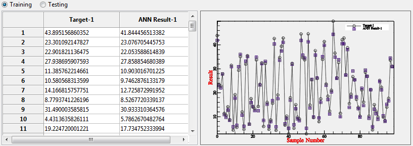
Anyway, after you finish “playing” with parameters, please click “Do Training”. And you should get the comparison of training data vs training result, checking data vs checking result, in form of table and chart as show in this example.

Using those kind of result comparison, it might be easier to decide whether the training is “enough” or still need more training process.

And also one of the important result from this training process is the Training logs that is printed in the bottom part of the software. This log basically tells everything about steps of training process, including the final result of weights and biases.

So, the training and checking is basically finished. But again, this procedure might need to be conducted back and forth with network setup to make sure of getting the best match to real data.

This is the end of this tutorial. Should anybody have question, please don’t hesitate to contact my email.
——————————————————————–
Written by Sugiyanto Suwono
Bekasi, April 30, 2013

Tutorial 2: AgielNN Network Preparation

Continuing the previous tutorial about data preparation, now we have 3 data, training, checking,and forecasting. In this tutorial, I will specifically discuss about how to create artificial neural network using those data.

To do that, please go to tab “Network Setup”, and you should find the blank panels in the right. The left most panel is training panel, while the middle panel is checking panel, and the right most panel is network diagram panel.

In the training panel, please select “Data-1 Training”. Since we want to use the first 2 column as input and last column as output, please select the appropriate column in the “Input” and “Output”. Repeat the procedure for Testing panel. Please remember, number of column selected in Training have to be equal to selected column in the Testing panel. However, if somehow you don’t have checking data, you could ignore the checking panel.

In the bottom of Training panel, there is an input of hidden layers. Please specify the preferred number of hidden layers. Each hidden layer must have hidden nodes inside it. The more hidden layers and hidden nodes each layer, the more complicated the network and the longer time to run the training. It is not guaranteed that the more number of hidden layers and nodes will give a better match during training. So, in the next training step, you should try to change this configuration to get the best match of neural network system.

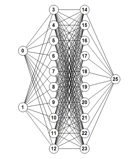
By pressing “Build Network”, you should get this kind of network in the right panel. This figure is an example of neural network diagram build using 2 input nodes, 2 hidden layers, 10 nodes in hidden layer 1 and 2, and 1 output node. Please notice that the “not shown” bullets like node number 2, 13, and 24 are biases node. Please refers to others detailed Artificial Neural Network tutorial to understand the term of bias and weight like in http://www.learnartificialneuralnetworks.com.

So, network preparation is basically finished. But, this procedure might should be conducted back and forth during training and checking to make sure of getting the best match to real data.


This is the end of this tutorial. Should anybody have question, please don’t hesitate to contact my email.
——————————————————————–
Written by Sugiyanto Suwono
Bekasi, March 13, 2013

Tutorial 7: Building Cross Plot

Cross section generally is a comparison of many log plot in a single viewer. It mostly used for correlation of zone penetrated by wells in order to understand the stratigraphic view of an oil and gas reservoir. So, to build a cross section, every well log plot must be generated. However, you don’t have to go to log plot panel since the cross section panel can handle everything by itself. However, some advance feature like editing zone and viewing data of log from log plot still unsupported in cross section panel.

LogView++ Cross Section


Add New Plot
To create a plot in cross section panel, go to “Well Plot” tab in the left part of cross section panel and click button (+). The following dialog will be prompted. Fill up all properties of the plot i.e. the name to the plot (only used for identifier, no effect to plot), depth mode whether TVD or MD Select the well to be plotted and also its log data, lithology package, and completion package. You also have to select the template to be used for plot. To plot only a certain depth, check “Use Custom Depth” and fill out the top and bottom depth.


Edit Existing Plot
If you made a mistake when creating a plot, you still can edit the plot by clicking button (…) in the “Well Plot” Tab. A similar dialog will also be shown up. Edit it and click OK to update.


Changing Order of Plot
The order of plotting in cross section from left to right is determined by the order of plot name in the plot list. To move to the right, click button “Down” while move to left by clicking button “Up”.


Delete Existing Plot
To delete the existing plot, click button (x) and confirm the deletion dialog.


Select Zone to Show
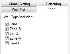
Zone is one of the most important thing in cross section. To show or hide the zone, you can simply check or uncheck the zone list in the “Zone” tab.


Choose Flattening Mode
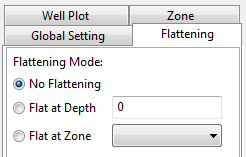
Flattening mode is very important in correlating plots. In most cases, using TVD mode and flatten to contact or a zone is recommended to compare the plot. However, LogView++ give you freedom to choose the flattening mode whether no flatten, use depth, or use zone. No flattening means every plot will be plotted as it is based on the data available in the plot (either las, lithology, its completion, or its custom depth). Flatten to depth means that t selected depth, the plot will be equal in position. While flatten to zone means that cross section will equalize all plot at selected zone in every well. In case of no zone available in a plot or well, the plot will be drawn from zero position at top of cross section position.


Use Global Setting
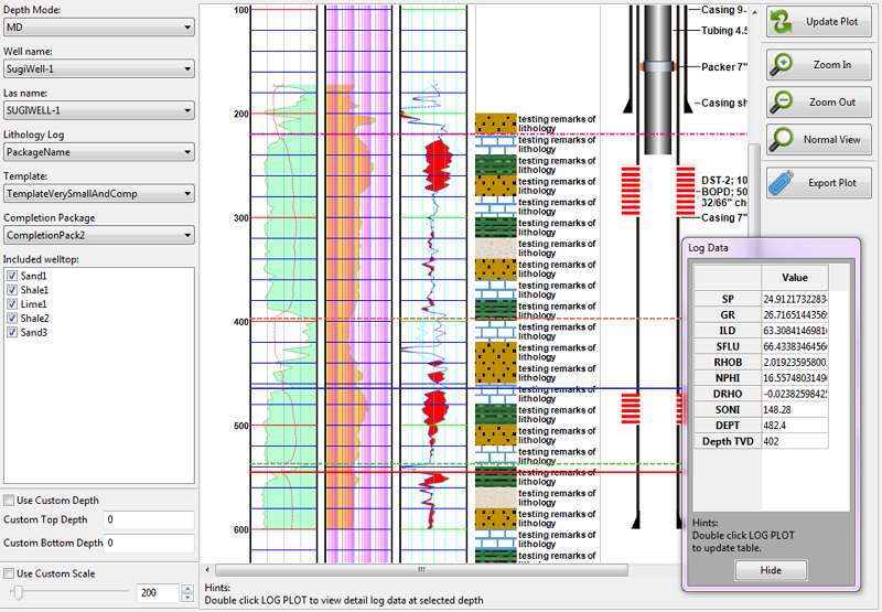
In case of you have created several plot in cross section but each plot have a different setting especially depth mode, Template, custom depth; you can force every plot to use a same setting using global setting. To do that, go to “Global Setting” panel and change the global depth mode, global template, and global custom depth. You can even change the scale of log by checking “Use Custom Scale” and fill the value of custom scale. After that click “update Plot” button in the right part of the cross section panel.


Changing Cross Section View
The plot can be modified by zooming.. Zooming in and out will only change the size of view, but not the bitmap of plot itself. So, just click button Zoom in or Zoom out in the right part of the cross section panel and everything should be done.


Exporting Cross Section
For further usage, some people probably need to make a screenshot of the plot to open it in a image viewer, or included it into a report file or something else. The easiest way to do that is by exporting the plot to a bitmap file. by clicking the button export plot you will be prompted with saving file dialog. Fill the file name and click ok.

Tutorial 6: Managing Log Plot

One of the most important feature of LogView++ is certainly the Log Plot. Since the first version of LogView++, it has been the main function of LogView++. The concept of log plotting is basically very simple.. A log plot should contain following data:

  • log asci data (las or asci file)
  • completion package
  • lithology package
  • plot template, and
  • well top

All of those data should be managed outside of log plot panel.. Log asci data should be conditioned in the log editor panel. Completion package is editable in the completion editor. Lithology package is also editable in Lithology editor. Template is a complicated data that must be managed in template editor. Meanwhile well top should also be managed in the zone editor. Once every data is ready, log plot panel should be able to use the data to create plot.


Creating Log Plot
Make sure to select MD or TVD mode for depth scale. After that, select well name exists in the project. Once well has been selected, available log data will be listed in log data combo box. Lithology and completion package will also be listed in the following combo box. Select those three data if available. At least one data must be exists to make sure that plot will be generated. After that, by selecting a template, the log plot will be filled with generated bitmap. To show zone in the plot, check well top available in the list.

Log Plot


Changing Plot View
The plot can be modified by changing the global scale value, using custom depth or zooming.. Increasing the scale will reduce the height of the plot. Changing the scale should be followed by refreshing the plot since it need to regenerate the bitmap. This scale value is actually a property of template. So, changing the global scale will temporarily overwrite the scale value of the template but not saved in the template. Using a custom depth will limit the viewer to plot only the interval of selected depth. Since it will regenerate the bitmap, you also need to click refresh button to update the plot after selecting custom depth. Zooming in and out will only change the size of view, but not the bitmap of plot itself.


Exporting Plot
For further usage, some people probably need to make a screenshot of the plot to open it in a image viewer, or included it into a report file or something else. The easiest way to do that is by exporting the plot to a bitmap file. by clicking the button export plot you will be prompted with saving file dialog. Fill the file name and click ok.


Viewing Detail LogData from Plot
At normal zoom mode, you can read the depth of the plot by hovering the mouse over the plot. The depth will be shown in the status bar. For further detail Log data, you can double click the plot. A dialog will be prompted to show the detail data at double-clicked depth.


Edit Well Top from Plot
Log Plot panel is also usefull to directly edit the well top penetrated by the well. By dragging the well top to a certain depth will automatically change the depth of well top and also overwrite the data of well top in the Zone Editor panel.

Tutorial 5: Template Management

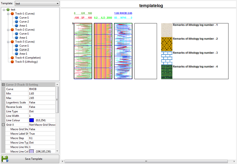
Template is a complex document that is very important to make a plot or cross section. The document of template should contain several properties depend on the number of track, number of curve on each track, and number of area on each track. Following picture is the screenshot of template editor. Every template can be modified in this template editor. Template is actualy text file. So basically if you don’t like with Template Editor, you can manually edit a template by using text editor and then import in to LogView++. However, if you are not sure what you are doing, it is strictly recommended to edit template inside the template editor rather than in a text editor.

LogView++ Template


Create New Template
Before we can customize a template, of course we have to create a template first. To do that, go to menu “Log Template” and Click new template.. Done. A default template should now be ready of the main LogView++ project tree.

Menu Template


Import Template
To import a template, in the menu “Log Template” click import. Browse an appropriate template file and click Ok. If template is valid, the imported template should now be ready in the project.


Export Template
Still in menu “Log Template”, click Export, select template in the prompted dialog and click OK. Fill the file name and click Save in the file dialog to export the file.


Delete Template
To remove a template from project, go to main LogView++ project tree, right click the template and click delete. Click yes in the confirmation dialog and template will be deleted.


Rename Template
To rename a template from project, go to main LogView++ project tree, right click the template and click setting. Type the new name and click ok to update the name.


Editing Template Properties
Go To Template editor select template you want to edit. Tree of template content should now be generated in the left part of Template Editor Panel.

Adding New Track

Right click the template name in the Template Tree and click Add Track. There are 3 kind of track available in LogView++ 2014; Curve Track, Completion Track, and Lithology Track. Curve Track can only be used to draw curve from log data. Completion Track is a place for drawing completion data. Meanwhile Lithology track is only able to handle the lithology data. After adding the track, you will see an empty track now available for editing.


Removing Track

Track can be removed by right-clicking the track in the template tree and click Delete Track


Adding Curve to a Curve Track

Right click the track and click Add New Curve.

Remove Curve

Right click the curve and click Delete.

Add Area

Right click the track and click Add New Area.

Remove Area

Right click the area and click Delete.

Editing Property Value

Every template data, Track, Curve, Area, or Template itself have many unique properties that will be used in log plotting.
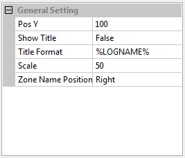
Properties of Template

      • Pos Y
        It is the Y position of the plot. Pos Y is calculated from the top position. So the higher the Pos Y the lower the position of the plot.
      • Show Title
        It is the choice whether you will show the plot title or not.
      • Title Format It is the format of the plot title. There are constant format that you can use for plotting specific data in LogView++ such as:
        Code
        Usage
        %WELLNAME% To show the well name
        %LOGNAME% To show the log name
        %LITHONAME% To show the lithology package name
        %COMPNAME% To show the completion package name

        Other than that, the text will be directly plotted.

        Example:
        MyWell:%WELLNAME%
        Will be printed as:
        MyWell:SUGI_WELL1
        In which SUGI_WELL1 is my real well name.

      • Scale
        It is the scale of the plot. The bigger the scale the shorter the plot.
      • Zone Name Position
        There are 2 places of zone name to plot. In the right or left.

Properties of Track

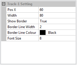
      • Pos X
        It is the X position of the track. X position is calculated from the left side of the plot. Higher value of X position the track will be plotted more right.
      • Width
        It is the width of track.
      • Show Border
        It is the option whether the border will be shown or not.
      • Border Line Width
        It means the thickness of the border line.
      • Border Line Colour
        It means the color that will be used for border.
      • Font Size
        It is the size of the font, especially for drawing its label
      • Width of Well (only available for completion track)
        Completion track will be divided into two column, the well column and label column. The width of well will be used to draw the well completion. The rest of (Width-Width of Well) will be used to draw the label. If Width of Well >= Width then label won’t be drawn.
      • Width of Lithology (only available for lithology track)
        Lithology track will also be divided into two column, the lithology column and label column. The width of lithology will be used to draw the lithology data. The rest of (Width-Width of Lithology) will be used to draw the label. If Width of Lithology >= Width then label won’t be drawn.

Properties of Curve

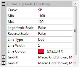
      • Curve
        It is the name of the curve to be plotted. The name of the curve have to be EXACTLY SIMILAR to the name of column in the log data.
      • Min
        It is the minimum scale of the curve. Any log value below minimum value will be plotted outside the track or technically ignored.
      • Max
        It is the maximum scale of the curve. Any log value above maximum value will be plotted outside the track or technically ignored.
      • Logaritmic Scale
        If the value is true, the curve will be drawn in logaritmic. Otherwise, the curve will be plotted in linier scale.
      • Reverse Scale
        In normal mode, the minimum scale would be in the left and maximum in the right position. For reverse mode, it would be in the backward position.
      • Line Type
        The line type could be SOLID, DOT, SHORT DASH, LONG DASH, or DOT & DASH.
      • Line Width
        It is the thickness of the curve line.
      • Line Colour
        It is the color of the curve line.
      • Grid-X and Grid-Y
        Grid X and Y properties will control the gridding process in the track. However, it is a part of curve property. So, in one track we can create more than one grid types. Grid-X will control grid in X direction (curve scale), while Grid-Y will control the Y direction (depth scale). Every grid consist of Macro and Micro grid. The Macro should have larger steps than the micro.

        • Macro Grid Shown
          It is the option whether to show the macro grid or not.
        • Macro Label Shown
          It is the option whether to show the macro grid label or not.
        • Macro Step
          It is the stepping value of Macro grid.
        • Macro Line Type
          It is the line type of Macro grid. It could be SOLID, DOT, SHORT DASH, LONG DASH, or DOT & DASH.
        • Macro Line Width
          It is the thickness of the Macro grid.
        • Macro Line Colour
          It is the Macro grid line color.
        • Micro Grid Shown
          It is the option whether to show the micro grid or not.
        • Micro Label Shown
          It is the option whether to show the micro grid label or not.
        • Micro Step
          It is the stepping value of Micro grid.
        • Micro Line Type
          It is the line type of Micro grid. It could be SOLID, DOT, SHORT DASH, LONG DASH, or DOT & DASH.
        • Micro Line Width
          It is the thickness of the Micro grid.
        • Micro Line Colour
          It is the Micro grid line color.

Properties of Area

      • Curve Left
        It is the name of curve as left border of the area. The curve name must be EXACTLY SIMILAR to the column name in the log data. if you want to plot area from the left border instead of a curve, use $LEFT_BORDER.
      • Curve Right
        It is the name of curve as right border of the area. the curve name must be EXACTLY SIMILAR to the column name in the log data. If you want to plot area to the right border instead of a curve, use $RIGHT_BORDER.
      • Fill Colour
        It is the fill color that will be used to draw the area.

Saving Edited Template

Before edited template could be used for any plot, the template must be saved first. To do that, click the button “Save Template” in the bottom part of the template editor. Or, if you accidentally open another panel, a saving dialog confirmation will be prompted. just click Yes to save it.

Tutorial 4: Well Completion Management

Completion data is an important feature in logview especiallyfor plotting the well sketchi the logplot or cross section panel. Completion data usually consist of casing, tubing, packer, and etc. In most cases, an oil or gas well will encounter any of workover or well service during its life period. Therefore, there should be more than one of completion package available in a well. Deal with that fact, LogView++ have been utilized with a capability to handle multiple completion package. Ok.. so the first thing need to be done on managing completion data is creating the completion package.


Create New Completion Package
To create the package, it can be simply done by clicking menu “Completion Data” and select “New Package”. A dialog showing package name will be prompted. Click ok to create the package. After that, an empty completion package should now be exists in the selected well.


Add Tool to Package
Once completion package is ready, tool can be added to the package. Go to panel Completion Editor, and click button “New Tool”. A dialog of tool selection will be prompted. Select the tool category and its specification (size). Click ok to add the selected tool. After that, a new tool should now be listed in the completion tool table.


Edit Specific Tool in Package
Double click specific tool in table. Fill editable properties. Done


Delete Tool from Package
Deleting tool is an easy task. Just click button “Delete Tool” and its simply done.


Export Package
The easiest way to use the completionpackage to an external software or to be reimported to another logview project is by exporting it to an asci file. Go to menu bar “Completion Data”and select Export Package. A file saving dialog will be prompted. Fill the file name and select save. You should now have a text file filled with tab delimited data of completion tools.


Import Package
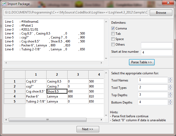
Importing is a backward step of exporting. It can also be simply done by selecting menu “Completion Data” and select Import Package. Browse the file and click ok. A completion parser dialog will be shown up. Select the delimiter, click Parse Table and select the appropriate column for tool name, depth start, depth end, and its tool type. Click next for final checking.

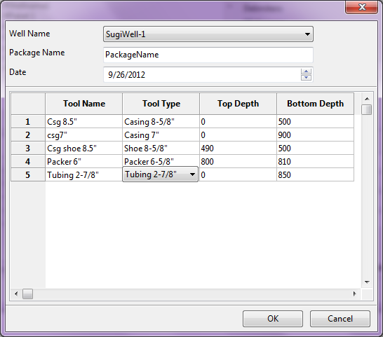
If every tool types are exists in the database, you can continue the wizard by clicking ok.. if not, you have to select the appropriate tool type in the database for each tool. Fill the incomplete data. Click OK and done.


Delete Package
To delete a completion package, go to main LogView++ project tree, right click a completion package and click delete. OK and done

Tutorial 3: Zone / Well Top Management

Well top is a marker of zone that has been penetrated by well. In logview++, it will be plotted in log plot window and cross section window.


Create New Zone
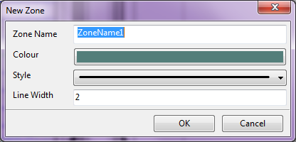
Well top can be created by accessing menu zonation and click new zone. A dialog will be prompted. Fill all properties; zone name, line width, line type, and line color, and then click ok to continue. A new zone will now exists in the main LogView++ project tree. In the panel of zone editor, you will see a table with new zone name and well name.


Delete Zones
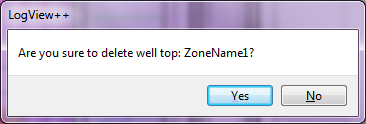
To delete a zone from project, Right Click Zone Name in the main project tree, and click Delete. Confirmation dialog will be shown up..


Edit Zones Properties
To edit the zone name, its line width, line style, and its color, right click zone name in the main project tree and click setting. An editing dialog will be prompted. Edit each property and click ok to update the property.

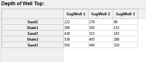
The most important property of well top is its depth position in every well. To edit it, go to panel zone editor and fill the depth in the table. In most cases, well top is recommended to be edited in TVD mode.. However, logview++ will save the MD data to make sure that a single depth especially for horizontal well that might have multiple TVD value for one value of MD. Consequently, if trajectory of the well is changed, the depth of TVD well top will be recalculated and overwritten.

!!!IMPORTANT!!!
Depth of -999.25 will be ignored. In case you really need that number, please give a bit change like -999.251.

Easier way to edit the depth of well top is by directly editing via log plot panel. By showing well top in log plot, at normal zoom mode, well top can be edited by dragging the well top (line) to a specific depth. By doing that, automatically the depth will be changed and the table of zone editor will also be refreshed.

It must be noted that LogView++ support only one depth data of each well for every well top. Therefore, in case of there is a fault penetrated by well that causes multiple depth of a well top in a single well, I recommend you to create a new different zone as a twin zone.


Import Zones
In case of you have a well top data, you can create a well top file in a text editor with format: WellTopName1, Depth@well1, Depth@well2, Depth@wellx, etc..

Example:
#WELLTOPS, WellName1, WellName2
NewZone1, 784, 778
NewZone2, 800, 798
NewZone3, 810, 806
NewZone4, 825, 831

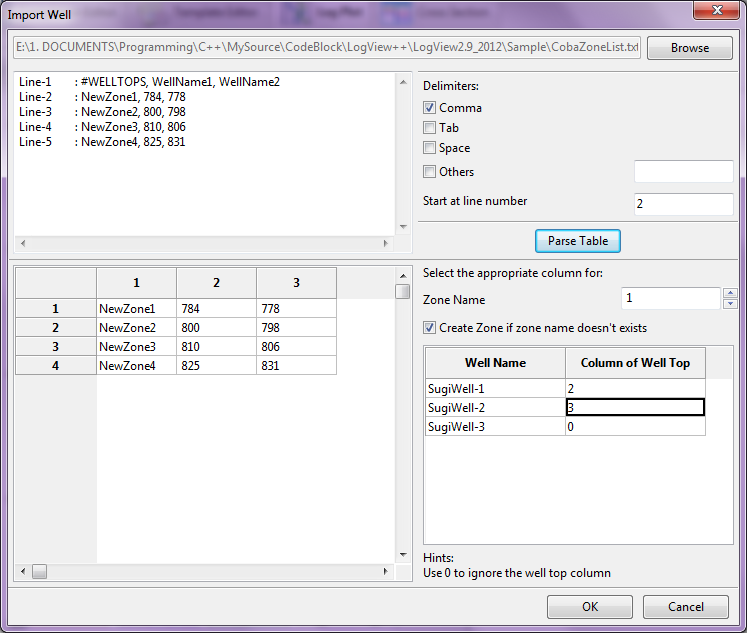
That formatted file can be directly imported to LogView++ thru menu Zonation and click import well top. A wizard dialog will be shown up. Browse the file, select the appropriate delimiter and the start line of the data and click Parse Table. After that, select the column of depth data for each existing well in the project. If the file doesn’t cover the depth data of a specific well, let it as default (0) which means to be ignored. You can also choose whether non-existing well top will be created or not. After click ok, a bunch of zone and its data should now be ready in the project.


Export Zones
Exporting well top is an easy way to create a delimited text file of the well top data. The format of generated file is similar to imported well top data file and described above.